
Introduction
There is a disconnect in mineral exploration between the data we collect, how we use it, and our goals. That disconnect results in a lot of wasted money and effort. There is a better way to explore systematically, to really use the data we collect, and to pursue the goals and constraints we have for a deposit – by using a targeting model.
A targeting model is an integrated 3D representation of geoscience data and project goals. It is a dynamic, 3D model that shows where to drill next based on your current information. It aggregates your geological data to give you a score to help prioritize drilling.
In this post, I’m going to talk about what a targeting model looks like and does. Then I’m going to use some historical data to demonstrate what a difference it can actually make.
Old idea, new approach
Of course, the idea of a targeting model is nothing new. The use of overlaid transparency maps to identify zones of interest dates back to at least the 1960s. Before that, however, the simple act of drawing a vein on a map was also a targeting model. The unmatched elegance and explanatory power of Conolly diagrams of vein thickness and grade are another kind of targeting model. Modern prospectivity models are excellent examples of targeting models, albeit ones that make the practice more complex than it perhaps ought to be.
When we all gather around and look at a long section or map together and say, “based on these things, we should drill here”, we are doing the same thing. But here’s the thing about models. The whole point is to get our shared ideas down into a single form that we can all look at. Because if we all have slightly different pictures in our heads, we will agree right up until the bullet hits the bone and then we will find out we were all thinking of something different.
What targeting models need to do
A targeting model has three jobs:
- Integrate the geological data that is important for exploration
- Include constraints such as minimum spacing between drillholes
- Clearly show the best place to drill, given that information and subject to those constraints
To build one, we need to identify and capture the links between our datasets and the project goal in order to make it operational. We collect a ton of data that is never seriously held to the test of “what do you actually tell me about where to drill next?”. Most of it tells us nothing. One of the best ways to understand the datasets you have is to build a targeting model, because it can clearly tell you what is useful and what is not.
Along with the input data, the model must enforce some constraints about the project (where to drill, how far apart, etc.), and puts it all into a simple package where 1 is good and 0 is bad. But it has one more critical feature: it must be dynamic. That means as new data is collected, and as new drillholes are added to the dataset, the model must update. Otherwise it is immediately out of date and useless.
Finally, and most importantly of all, the model must be immediately usable by actual practitioners in the software that they use every day.
So we’ve got something like Figure 1: a series of potential targets (in this case, blocks) scored by some combination of geoscience data and incorporating limits to spacing from existing drillholes.

The experiment
I want to show you just how much of a difference taking this kind of simple, systematic, integrated approach can make for a real project. To do that, I did an experiment using public data for the early stages of an historic exploration project. I wanted to compare the relative efficiency in drilling off a structure between what was actually done and what strictly using a targeting model could have saved.
I compiled a database for the project and made two versions: one frozen near the beginning of the project, and another with the full data from several subsequent years of exploration. At the start of the experiment, there was around 70 drillholes into the structure already.
I built my model in Leapfrog Geo using only the data available in the starting database. I used soil geochemistry, magnetics, drillhole lithology, drillhole geochemistry, and assays to build a geological model, then a targeting model (Figure 2).

I used the targeting model to decide where to drill using the score property. Once I had a set of targets, I turned on the real drillhole that was the closest to each target to “drill” it. Finally, I measured the volume of the structure within 25 m and 50 m of drilling to reflect the Indicated and Inferred categories applied in a later resource for the project.
I also performed the experiment again, this time ignoring the score property and just focusing on optimizing the geometry of the drillholes themselves. I wanted to see if the score property was actually helping or not.
Finally, I used the average volume defined per actual drillhole for the historic dataset for the structure as the “actual” value. I used the average because I don’t actually know the precise order in which the drillholes were drilled, but also because in reality the project was conducting exclusively even more closely spaced drilling than what I show here at the beginning of the experiment. I used the overall average, which is more representative of what actually happened, to avoid unfairly skewing the actual results with a phase that was clearly not about extending the resource.
Results
The results are shown in Table 1 and 2 where I compare the volume added by twenty drillholes from the actual drilling, the efficient spacing-only experiment, and the targeting model. The efficient spacing experiment and the targeting model both resulted in increased efficiency, defined as volume defined in the resource per drillhole.
Table 1: Drilling off structure at 25 m spacing (Indicated)
| Scenario | Volume defined (m3) | Drillholes | Volume per drillhole (m3) | Efficiency ratio |
|---|---|---|---|---|
| Actual | 455,000 | 20 | 23,000 | 1.0 |
| Efficient spacing | 631,000 | 20 | 32,000 | 1.4 |
| Targeting model | 1,071,000 | 20 | 54,000 | 2.3 |
Figure 3 shows the same data as cumulative Indicated volume added per drillhole for each of the three scenarios.

As expected, the volume per drillhole is higher for inferred because of the < 50 m spacing constraint. The efficiency ratio is higher too, because portions of the structure were drilled at closer spacing from the beginning in the actual program.
Table 2: Drilling off structure at 50 m spacing (Inferred)
| Scenario | Volume defined (m3) | Drillholes | Volume per drillhole (m3) | Efficiency ratio |
|---|---|---|---|---|
| Actual | 647,000 | 20 | 32,000 | 1.0 |
| Efficient spacing | 1,834,000 | 20 | 92,000 | 2.9 |
| Targeting model | 2,873,000 | 20 | 144,000 | 4.5 |

Table 3 shows the effect on project costs for the entire structure for the more conservative <25 m Indicated constraint. The actual volume added to the structure during the year after the dataset was frozen was 2,000,000 m3 in Indicated and 3,000,000 m3 in Indicated and Inferred. During that time, just over 90 drillholes were drilled prior to a resource estimate on the structure. I assumed the efficiency ratio between the efficient spacing and targeting model methods was constant and calculated the number of holes that would be required for each scenario. Then I used the more conservative 25 m spacing results, the actual average drillhole length (175 m), and the inflation-adjusted drilling cost (420 $/m) to calculate the cost and potential savings. The results are shown in Table 3.
Table 3: Savings due to increased efficiency at 25 m spacing
| Scenario | Efficiency ratio | Holes drilled | Cost (CAD) | Savings (CAD) |
|---|---|---|---|---|
| Actual | 1.0 | 92 | $6,762,000 | $0 |
| Efficient spacing | 1.4 | 66 | $4,851,000 | $1,911,00 |
| Targeting model | 2.3 | 40 | $2,940,000 | $3,822,000 |
The targeting model would have delivered the same amount of coverage and resource volume for less than half of the drilling. That’s a savings of more than $3.5M CAD in just one year using an inflation-adjusted cost per m. Careful control of spacing while ignoring the score resulted in an impressive savings on its own of almost $2M, although it benefited from the construction of the input datasets for the targeting model too.
Discussion
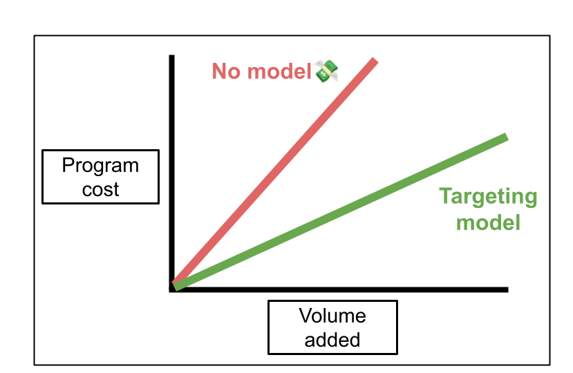
Targeting models make systematic, goal-oriented drilling easier and deliver real project savings by getting more done for less.
This study introduced no new data to the project. It was all completed using existing data, and was just a matter of getting it together into a model. Actually using geology information in targeting is a big problem, though, because it’s hard to look at many datasets at once. In reality, the industry tendency is to add more data to the pile without taking a critical look at how it is used.
Effective drill spacing alone would result in huge efficiency gains, but adding geology information makes sure you’re testing a model and using your data too. Systematic spacing does a lot of the work on its own, but it is surprisingly difficult to do that even in the artificial setting of this experiment, let alone justify in real life. A score property, reflecting the datasets I would have wanted to look at anyways all combined together into a single value, made it simple. There was a slight increase in average grade for the holes in the targeting model scenario, but overall it was similar to the overall average for the other holes in the structure.
One last thing. I used public data here and I don’t want to go into the specifics of the project or identify it. The people who worked on it did an excellent job and were very successful. This is just zooming in to one particular part to look at a specific scenario. If anything, the quality of historic work set a very high bar for any model to clear, which makes me more confident in the overall results.
Conclusion
So now we can agree on what a targeting model is and how they make exploration much more efficient: by focusing on our real goals, and by ensuring that drilling is as informative as possible. They need to be dynamic and usable in the software we use every day. And they need to clearly show where to drill.
The only progress we can make in exploration is through collecting more measurements of the true variable of interest: the 3D distribution of metal. And those measurements, collected through drilling, are not cheap. The goal for modelling should ultimately be to become more efficient with that significant cost so that we can drill more.
The experiment demonstrated that the potential gain from building a targeting model is significant, even for an already tightly-run project. The gain comes from being able to generate the same information for less – which means being able to drill more. To get there, we need to clearly define the project goals and couple them to the data we collect.
And if that sounds like a lot – feel free to reach out, because we do this all day.
Leave a Reply